QCBS workshop on the use of open source tools for advanced spatial analysis
April 16 2019, McGill University.
Installation of software
Installation of PostGIS
For Windows and Mac users
- Install PostgreSQL from the EntrepriseDB website EntrepriseDB
- When asked if you want to install Stackbuilder, choose yes and select to install PostGIS under “spatial extensions”. When you are asked, choose to create a new spatial database and name it spatiadb. Answer yes to questions about GDAL_DATA, POSTGIS_GDAL_ENABLED_DRIVERS, POSTGIS_ENABLED_OUTDB_RASTERS.
For Linux users (Ubuntu/Debian)
sudo apt-get install postgresql postgis
Then type
sudo gedit /etc/postgresql/11.2/main/postgresql.conf
remove the # in front of #listen_addresses = 'localhost'
restart postgresql
sudo service postgresql restart
For Mac users. In the psql terminal, type:
SHOW hba_file;
You then need to edit the postgresql.conf file to remove the # in front of #listen_addresses = 'localhost'. You can also Put Trust at the end of the lines with localhost.
To create a spatial database
CREATE DATABASE spatialdb;
\c spatialdb;
CREATE EXTENSION postgis;
CREATE EXTENSION postgis_topology;
Data for exercises
Click here to download datasets that will be used for this workshop. Note that all files are in the Latitude/Longitude (datum WGS84) CRS.
- obis_toothed_whales.shp → Occurrences of toothed whales downloaded from the OBIS(http://iobis.org/) website.
- world_bedrock_topo.tif → Topography of the earth surface, downloaded from here: http://www.ngdc.noaa.gov/mgg/global/global.html
- EEZ_IHO_union_v2.shp → Union of the marine ecozones and “Exclusive Economic Zones Boundaries” (EEZ) downloaded here http://www.marineregions.org/downloads.php
- TM_WORLD_BORDERS-0.3.shp → World political borders, downloaded here: http://thematicmapping.org/downloads/world_borders.php
- meow_ecos.shp → Marine Ecoregions of the World (MEOW), downloaded here [http://www.marineregions.org/downloads.php]]
Using PostGIS with QGIS
Import data from QGIS to PostGIS
- Click on Layer…Add Layer…Add PostGIS layer.
- Click on New to create a new connection.
- Give a name to the connection (“qcbs_workshop”), specify “localhost” as the host, “spatialdb” as the database, and specify your user name (usually “postgres”).
- Make sure that you have the DB Manager extension activated in the list of plugins.
- In the top menu, go to Database… DB Manager. Click on PostGIS and navigate to the spatial database (spatialdb) that you created.
- Click on the Import Layer/File icon and choose the file “obis_toothes_whales.shp”. Choose “Create spatial index” and “Create singlepart geometry insted of multipart” and leave the other options unchanged. Name the table “obis_whales”, in lowercase. Remember that table names in PostgreSQL must be in lowercase and should not contain spaces, special characters or accented characters.
- Repeat these steps for EEZ_IHO_union_V2.shp (name it eez_iho), meow_ecos.shp (name it meow) and TM_WORLD_BORDERS.shp (name it tm_world). Choose “Create spatial index” BUT DON'T SELECT “Create singlepart geometry insted of multipart” for these polygon layers.
- Note that you might have to click the refresh icon to see the new layers appearing in the DB Manager.
Functions for basic queries on single layers
sum(expression) aggregate to return a sum for a set of records
count(expression) aggregate to return the size of a set of records
ST_GeometryType(geometry) returns the type of the geometry
ST_SRID(geometry) returns the spatial reference identifier number of the geometry
ST_X(point) returns the X ordinate
ST_Y(point) returns the Y ordinate
ST_Length(linestring) returns the length of the linestring
ST_StartPoint(geometry) returns the first coordinate as a point
ST_EndPoint(geometry) returns the last coordinate as a point
ST_Area(geometry) returns the area of the polygons
ST_Perimeter(geometry) returns the length of all the rings
ST_AsSVG(geometry) returns SVG text
ST_Transform(geometry, SRID) change the reference system from the current one (of geom) to the one defined by SRID.
Select all observations North of the 70th parallel
SELECT * FROM obis_whales WHERE latitude > 70
Select all observations South of the 60th parallel
SELECT tname, latitude FROM obis_whales WHERE latitude < -60
List the species that can be found South of the 60th parallel
SELECT DISTINCT tname FROM obis_whales WHERE latitude < -60
Create a new layer, with belugas only
CREATE TABLE belugas AS SELECT * FROM obis_whales WHERE tname='Delphinapterus leucas'
Area of each country, sorted in decreasing order and calculated in square kilometers.
SELECT name, ST_Area(geography(geom))/1000000 as areakm2 FROM tm_world ORDER BY area DESC
Area of each sea, sorted in decreasing order. Note that there can be many polygons in eez_iho for each sea, so we need to use a GROUP BY clause.
SELECT iho_sea, sum(ST_Area(eez_iho.geom)) as area FROM eez_iho GROUP BY iho_sea ORDER BY area DESC
Extract latitudes and longitudes of each occurrence of “Delpinus delphis”.
SELECT ST_X(geom), ST_Y(geom) FROM obis_whales WHERE tname='Delphinus delphis'
Distance to the nearest neighbour beluga for each beluga occurrence location
SELECT DISTINCT ON(a.id) a.id, b.id as nn_id, ST_Distance(a.geom,b.geom) as dist FROM obis_whales a, obis_whales b WHERE a.id <> b.id AND a.tname='Delphinapterus leucas' AND b.tname='Delphinapterus leucas' ORDER BY a.id,dist
EXERCISE 1 Find the country that has the biggest ratio between the square root of it's area and its perimeter. Which country has the smallest ratio?
EXERCISE 2 Extract the X and Y coordinates in the CRS WGS 84/World Mercator (EPSG: 3395) of the only individual of “Electra” in the dataset.
Spatial relationship between layers
ST_Contains(geometry A, geometry B): Returns true if and only if no points of B lie in the exterior of A, and at least one point of the interior of B lies in the interior of A.
ST_Crosses(geometry A, geometry B): Returns TRUE if the supplied geometries have some, but not all, interior points in common.
ST_Disjoint(geometry A , geometry B): Returns TRUE if the Geometries do not “spatially intersect” - if they do not share any space together.
ST_Distance(geometry A, geometry B): Returns the 2-dimensional cartesian minimum distance (based on spatial ref) between two geometries in projected units.
ST_DWithin(geometry A, geometry B, radius): Returns true if the geometries are within the specified distance (radius) of one another.
ST_Equals(geometry A, geometry B): Returns true if the given geometries represent the same geometry. Directionality is ignored.
ST_Intersects(geometry A, geometry B): Returns TRUE if the Geometries/Geography “spatially intersect” - (share any portion of space) and FALSE if they don’t (they are Disjoint).
ST_Overlaps(geometry A, geometry B): Returns TRUE if the Geometries share space, are of the same dimension, but are not completely contained by each other.
ST_Touches(geometry A, geometry B): Returns TRUE if the geometries have at least one point in common, but their interiors do not intersect.
ST_Within(geometry A , geometry B): Returns true if the geometry A is completely inside geometry B
Extract the id and the names of the toothed whales and the name of the sea in which they are found in Canadian waters.
SELECT a.id, a.tname, b.iho_sea FROM obis_whales a, eez_iho b WHERE ST_Within(a.geom,b.geom) AND b.country='Canada'
Count the occurrences of each species of toothed whale in Canadian waters.
SELECT a.tname, count(*) as num FROM obis_whales a, eez_iho b WHERE ST_Within(a.geom,b.geom) AND b.country='Canada' GROUP BY a.tname ORDER BY num DESC
Select all toothed whale occurrences that are closer than 1 degree from the Canadian land border.
SELECT a.* FROM obis_whales a, tm_world b WHERE ST_DWithin(a.geom,b.geom,1) AND b.name='Canada'
You can click on “Load as layer” and “Load now” to view it in QGIS. This might take a while…
Create a new polygon representing a buffer zone of 100 km around Australia. Note that we need to convert it to Multipolygon because QGIS doesn't understand the Polygon type.
CREATE TABLE aus_buffer AS
SELECT ST_Buffer(geography(geom),100000)::geometry(Multipolygon,4326) AS geom
FROM tm_world
WHERE name='Australia'
EXERCISE 3 - Calculate the number of occurrences of toothed whales per month in UK waters (table eez_iho). Use the function EXTRACT from PostgreSQL to extract the month from the datecollec column. To convert text column containing a date to a data type use ::date (datecollec::date).
EXERCISE 4 Of the countries that have a surface area of less than 20,000 km2 (2e+11 m2), which of them has the largest number of toothed whales within 1 degree of their frontiers?
Challenge Create a new table with all toothed whale occurrences in the Polar latitudinal zone and situated North of the Equator. Visualize these observations with the North_Pole_Azimuthal_Equidistant CRS in QGIS on top of the TM_Word_Borders shapefile.
Using PostgreSQL/PostGIS, GDAL, sf and GRASS in R
Download the R file containing the code for this part of the workshop
- Package rpostgis
- Package RQGIS3
- Package rgrass7
- Package RPostgreSQL
- Package rgdal
- Package sf - Simple Features
Using the Processing Framework in QGIS
You first need to install the Processing R Provider plugin in QGIS. Then, restart QGIS!
Commands to specify the input and output files and script options in Processing
raster. A raster layer.
vector. A vector layer.
table. A table.
number. A numerical value. A default value must be provided. For instance, depth=number 2.4.
string. A text string. As in the case of numerical values, a default value must be added. For instance, name=string Victor.
boolean. A boolean value. Add True or False after it to set the default value. For example, verbose=boolean True.
multiple raster. A set of input raster layers.
multiple vector. A set of input vector layers.
field. A field in the attributes table of a vector layer. The name of the layer has to be added after the field tag. For instance, if you have declared a vector input with mylayer=vector, you could use myfield=field mylayer to add a field from that layer as parameter.
folder. A folder.
file. A filename.
To create a new R Processing script, click on the R logo on the top of the processing toolbox pane, and select Create New R Script. When you are done typing the script, give it an appropriate name and save it in the default folder that opens.
Exercice 5
Create a new R script in the toolbox by copying and pasting this Processing/R script that creates 100 points distributed randomly on the earth in the latitude/longitude reference system (EPSG 4326) and that are imported as a QGIS layer.
Overlay the result on top of the TM_World_Borders shapefile.
Exercice 6
Create a script that loads the TM_WORLD_BORDERS file in R, calculates the area with st_area and plots the log-log relationship between area and population (POP2005 column). Add the country names as labels.
Exercice 7
Create a user interface that allows selecting the country and sea layers as well as specifying the name of a country, and obtaining a bar plot showing the area of each sea situated within 0.5 degrees of the chosen country. Note that you need to add the layers TM_WORLD_BORDERS and EEZ_IHO_union_v2 to the QGIS canvas
1 - Open the Processing toolbox, click on R script…Tools…Create New R Script.
2 - Copy-paste the following code in the R script and save it under Countries_Zones_Plot. This code will take the final polygon layer containing each sea in the buffer around the chosen country and create the barplot.
##QCBS Workshop=group
##Layer=vector
##showplots
#data2=tapply(Layer$new_area,Layer$IHO_Sea,mean)
library('dplyr')
Layer=data.frame(Layer)
data2=Layer%>%group_by(IHO_Sea)%>%summarize(mean=mean(new_area))
par(mar=c(10,4,4,2))
barplot(data2$mean, names.arg=data2$IHO_Sea, las=2)
3 - Open the “Graphical Modeler”
4 - Specify “Country seas” as the name of the model and “QCBS Workshop” as the group.
5 - Add a vector layer to the model, name it “Countries” and specify polygon as the “geometry type”.
6 - Add a “String” to the model and name it, “Country Name”.
7 - Add “Extract by attributes” to the model (under Algorithms>Vector selection). Specify “Countries” as the “Input Layer”, = as the operator, NAME as the “Selection Attribute”, click on the Gear icon under Value, choose Model input and select “Country Name” as the “Value”.
8 - Add a “Buffer” to the model. Specify “Output from Extract by Attributes” as the “Input”, and specify the distance as 0.5 (it's in degrees since the map is in latitude/longitude). Choose to “dissolve the output” and leave other field blank.
9 - Add another Vector Layer to the model. Name it “Sea Zones”. Specify “Polygon” as the “shape type”. This will be our polygons layer containing the different seas.
10 - Add “Intersection” to the model. Specify an intersection between “Buffered from Buffer” and the layer “Sea Zones”. Leave other field blank.
11 - Add “Field Calculator” to the model. Choose the intersection layer from the previous step as the input. Specify new_area as “Result Field Name” and $area as the fomula. This will calculate the area of each polygon of each section of sea in the buffer zone around the country in degrees squared.
12 - Now, add the R script created at Step 2 to the model. “Input” is the output from Step 11 (Field Calculator). Call the output file “Country_seas”
Your model should look like this one:

13 - You are now ready to run the model! First, save the model and name it Country_seas. Then, close the “Graphical Modeler” and double-click on your model in the Toolbox under Models. Specify TM_World_Borders as the Country layer and EEZ_IHO_union_v2 for the zones. Specify the name of a country of your choice (ex. Canada).
14 - When the algorithm stops running, you should see a graphic showing the area of each sea along the coast of the country you chose.
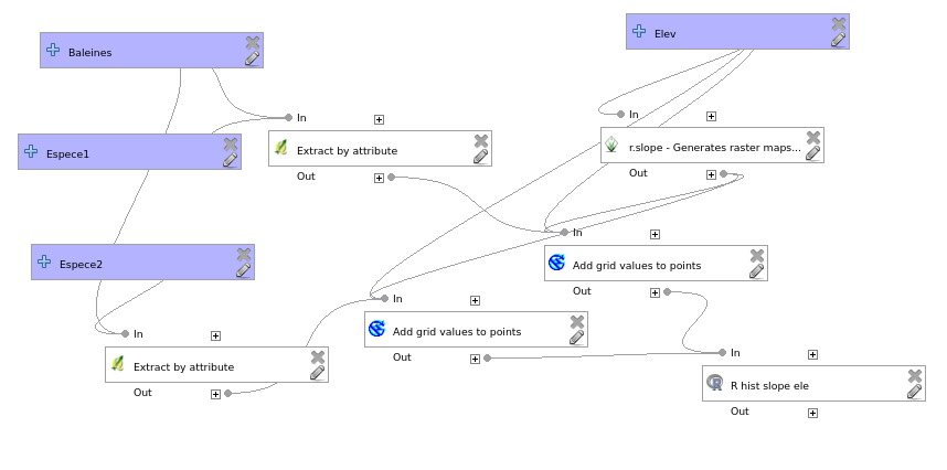
CHALLENGE
Create a graphical model in Processing to extract and compare the elevation and the slope for each occurrence of two species of toothed whales (that you choose in the interface) and to create histograms showing the distribution of slopes and elevation points of the two species from R. Use the fonction r.slope from GRASS and the function “Add grid values to points” from SAGA (in Shapes…points) in your model.